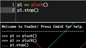
These paragraphs explore the concept of live coding and why it attracts people. As an interdisciplinary practice combining coding, art, and improvised performance, live coding appeals to both technicians and artists. It provides a unique medium to appreciate the beauty of coding and the artistic aspects often hidden within what is typically seen as a highly technical and inaccessible field.
I encountered live coding for the first time while working as a student staff member at ICLC2024. These performances gave me a basic understanding of live coding as a layperson. Reading this article later deepened my perspective and sparked new thoughts.
The article describes live coding as a way for artists to interact with the world and each other in real-time through code. Watching live coding performances, I initially assumed artists focused entirely on their work, treating the performance as self-contained and unaffected by external factors. However, I may have overlooked the role of the audience, the venue, and the environment in inspiring the artists and adding new layers to the improvisation. As someone who loves live performances, I now see live coding as another form where interaction between the artists and their surroundings is crucial.
The article also mentions how projecting code on the screen as the main visual makes the performance more transparent and accessible. While I agree with this, it also raises a concern. A friend unfamiliar with live coding once referred to it as a “nerd party,” commenting that it’s less danceable than traditional DJ performances and difficult for non-coders—or even coders unfamiliar with live coding languages—to follow. I wonder if this limits the audience’s ability to understand and fully appreciate the performance or the essence of the art form. Although this may not be a significant issue, it’s something I’m curious about.
The idea was to combine hydra visuals with an animation overlayed on top. Aadhar drew a character animation of a guy falling, which was used on top to drive the story and the sounds. Blender was used to draw the frames and render the animation.
The first issue that came up with overlaying the animation was turning the background of the animated video transparent. We tried really hard to get a video with a transparent background into hydra, but that didn’t work because the background showed up black at the end no matter what we did. Then, we used hydra code itself to turn the background transparent, using its luma function that was relatively easier to do.
Then, because we had a video that was 2 minutes long, we couldn’t get all of it into hydra. Apparently, hydra only accepts 15-second-long clips. So we had to chop it up into eight 15-second-long pieces and trigger each video at the right time to make the animation flow. However, it wasn’t as smooth as we thought it would be. It took a lot of rehearsals for us to get used to triggering the videos at the right time – which didn’t come off even till the end. The videos were looping before we could trigger the next one (which we tried our best to cover and the final performance really reflected it). Other than the animation itself, different shaders were used to create the background of the thing.
Chenxuan was responsible for this part of the project. We created a total of six shaders. Notably, the shader featuring the colorama effect appears more two-dimensional, which aligns better with the animation style. This is crucial because it ensures that the characters and the background seem to exist within the same layer, maintaining visual coherence.
However, we encountered several issues with the shaders, primarily due to a variety of errors during loading. Each shader seems to manifest its unique problem. For example, some shaders experience data type conflicts between integers and floats. Others have issues with multiple declarations of ‘x’ or ‘y’ variables, which cause conflicts within the code.
Additionally, the shaders display inconsistently across different platforms. On Pulsar, they perform as expected, but on Flok, the display splits into four distinct windows, which complicates our testing and development process.
The audio is divided into three main parts: one before the animation, one during the animation, and one after the animation. The part before the animation features a classic TidalCycles buildup—the drums stack up, a simple melody using synths comes in, and variation is given by switching up the instruments and effects. This part lasts for roughly a minute, and its end is marked by a sample (Transcendence by Nujabes) quietly coming in. Other instruments fade out as the sample takes center stage. This is when the animation starts to come in, and the performance transitions to the second part.
The animation starts by focusing on the main character’s closed eyes. The sample, sounding faraway at first, grows louder and more pronounced as the character opens their eyes and begins to fall. This is the first out of six identifiable sections within this part, and this continues until a moment in which the character appears to become emboldened with determination—a different sample (Sunbeams by J Dilla) comes in here. This second part continues until the first punch, with short samples (voice lines from Parappa the Rapper) adding to the conversation from this point onwards.
Much of the animation features the character falling through the sky, punching through obstacles on the way down. We thought the moments where these punches occur would be great for emphasizing the connection between the audio and the visuals. After some discussion, we decided that we would achieve this by switching both the main sample and the visuals (using shaders) with each punch. Each punch is also made audible through a punching and crashing sound effect. As there are three punches total, the audio changes three times from the aforementioned second part. These are the third to fifth sections (one sample from Inspiration of My Life by Citations, two samples from 15 by pH-1).
The character eventually falls to the ground, upon which the animation rewinds quickly and the character falls back upwards. A record scratch sound effect is used to convey the rewind, and a fast-paced, upbeat sample (Galactic Funk by Casiopea) is used to match the sped-up footage. This is the sixth and final section of this part. The animation ends by focusing back on the character’s closed eyes, and everything fades out to allow for the final part to come in.
The final part seems to feature another buildup. A simple beat is made using the 808sd and 808lt instruments. A short vocal(ish?) sample is then played a few times with varying effects, as if to signal something left to be said—and indeed there is.
Code for the audio and the lyrics can be found here.
Breakdown: Noah + Aakarsh worked on music mainly. Aakarsh made pt2,3,6,7,8 while Noah made pt 4,5. Nicholas made all the visual effects while the group decided the videos+text to be displayed mostly together.
The music is inspired by various hyperpop, dariacore, digicore and other internet-originated microgenres. The album’s Dariacore, Dariacore 2, Dariacore 3 by artist Leroy were particularly the inspirations in mind. People on the internet jokingly describe Dariacore as maxxed out plunderphonics and the ADHD-esque hyper intensity of the genre couple with meme-culture infused pop sampling was what particularly attracted me and noah. While originally starting as a Dariacore project, this 8-track project eventually ended up spanning multiple genres to provide narrative arcs and various downtempo-uptempo sections. This concept is inspired by Machine Girl’s うずまき (Uzumaki) , a song that erratically cuts between starkly different music genres and emotional feels. We wanted our piece to have a combination of this song’s composition and a DJ set as our composition. Here’s a description of the various sections: Here’s a description of various sections:
For the visuals, we wanted to incorporate pop culture references and find the border between insanity and craziness. We use a combination of real people, anime, and NYUAD references to keep the viewer guessing what’ll come next. I tried to get around Hydra’s restrictions when it comes to videos by developing my own FloatingVideo class that enabled us to play videos in p5 that we could put over our visuals. I also found a lot of use in the blend and layer functions that allowed us to combine different videos and sources onto the canvas.
For our visual side, we have decided to begin with vibrant visuals characterized by dynamic, distorted light trails. Our initial code included loading the image, modulating it with a simple oscillator, and then blending it with the original image, resulting in a blur effect. As we progressed, we integrated more complex functions based on various modulations.
As our project evolved, our goal was to synchronize our visuals more seamlessly with the music, increasing in intensity as the musical layers deepened. We incorporated a series of ‘mult(shape)’ functions to help us calm down the visuals during slower beats.
Finally, we placed all the visuals in an array and used CCV to update them upon the addition of each new layer of music. This enabled us to synchronize the transitions between the music and visuals. Additionally, we integrated CCs into the primary visual functions to enhance the piece with a more audio-reactive experience.
created an array of visuals that enabled swift transitions, all perfectly timed with sound triggers for perfect synchronization. Additionally, we integrated CC’s into the main visual functions to enhance the piece with a more audio-reactive experience.
For our final composition, our group created a smooth blend of UK Garage and House music, set at a tempo of 128 BPM. The track begins with a mellow melody that progresses up and down in the E-flat minor scale. On top of this melody, we layered a groovy UK Garage loop, establishing the mood and setting the tone of the composition.
To gradually introduce rhythm to our composition, Jeong-In layered various drum patterns, adding hi-hats, claps, and bass drums one by one. On top of Jeong-In’s drums, we introduce another layer of classic UK Garage drum loop, which completes the rhythmic structure of the composition.
Furthermore, we incorporated a crisp bass sound, which gave the overall composition a euphoric vibe. After introducing this element, we abruptly cut off the drums to create a dramatic transition. At this point, we added a new melodic layer, changing the atmosphere and breaking up the repetitiveness of the track. Over this new layer, we reintroduced the previously used elements but in a different order and context, giving the composition a fresh perspective.
Additionally, we used a riser to smoothly transition into our drum loop and also incorporated a sea wave sound effect to make the sound more dynamic. We end the composition with a different variation of our base melody, utilizing the jux rev function.
An important element of the practice of Live Coding is how it challenges our current perspective and use of technology. We’ve talked about it through the lens of notation, liveliness(es), and temporality, among others. Our group, the iCoders, wanted to explore this with our final project. We discussed how dependent we are on our computers, many of us Macs. What is our input, and what systems are there to receive this? What does 4 people editing a Google document simultaneously indicate about the liveliness of our computer? With this in mind, we decided to construct a remix of sounds in Apple computers. These are some of the sounds we hear the most on our day to day, and we thought it would be fun to take them out of context, break their patters, and dance to them. Perhaps a juxtaposition between the academic and the non-academic, the technical and the artsy. We wanted to make it be an EDM remix because this is what we usually hear at parties, and believe that the style would work really well. We began creating and encountered important inspirations throughout the process.
Techno:
Diamonds on my Mind: https://open.spotify.com/album/4igCnwKUaJNezJWHlWv8Bs
During one of our early meetings, we had the vast libary of apple sounds, but were struggling a bit with pulling something together. We decided to look if someone had done something similar to our idea and found this video by Leslie Way which helped us A LOT.
Mac Remix: https://www.youtube.com/watch?v=6CPDTPH-65o
Compositional Structure: From the very beginning we wanted our song to be “techno.” Nevertheless, once we found Leslie Way’s remix, we thought that the vibe that remix goes for is very fitting to Apples’ sounds. Upon testing and playing around with sounds a lot, we settled on the idea of having a slow, “cute” beginning using only (or mostly) Apple sounds. Here, the computer would get slowly overwhelmed with us from all the IM assignments and tabs open. The computer would then crash, and we would introduce a “techno” section. Then, we’d try to simulate a bit the songs that we’d been listening to. After many many many iterations, we reached a structure like this:
The song begins slow, grows, there is a shutdown, it quickly grows again and there is a big drop. Then the elements slowly fade out, and we turn off the computer because we “are done with the semester.”
Sound: The first thing we did once we chose this idea was find a library of Apple sounds. We found many of them on a webpage and added those we considered necessary from YouTube. We used these, along with the Dirt-Samples (mostly for drums) to build our performance. We used some of the songs liked above to mirror the beats and instruments, but also a lot of experimentation. Here is the code for our Tidal Cycles sketch:
hush
boot
one
two
three
four
do -- 0.5, 1 to 64 64
d1 $ fast 64 $ s "apple2:11 apple2:10" -- voice note sound
d2 $ fast 64 $ s "apple2:0*4" # begin 0.2 # end 0.9 # krush 4 # crush 12 # room 0.2 # sz 0.2 # speed 0.9 # gain 1.1
once $ ccv "6" # ccn "3" # s "midi"
d16 $ ccv "10*127" # ccn "2" # s "midi";
shutdown
reboot
talk
drumss
once $ s "apple3" # gain 2
macintosh
techno_drums
d11 $ silence -- silence mackintosh
buildup_2
drop_2
queOnda
d11 $ silence -- mackin
d11 $ fast 2 $ striate 16 $ s "apple3*1" # gain 1.3 -- Striate
back1
back2
back3
back4
panic
hush
-- manually trigger mackin & tosh to spice up sound
once $ s "apple3*1" # begin 0.32 # end 0.4 # krush 3 # gain 1.7 -- mackin
once $ s "apple3*1" # begin 0.4 # end 0.48 # krush 3 # gain 1.7 -- tosh
-- d14 $ s "apple3*1" # legato 1 # begin 0.33 # end 0.5 # gain 2
-- once $ s "apple3*1" # room 1 # gain 2
hush
boot = do{
once $ s "apple:4";
once $ ccv "0" # ccn "3" # s "midi";
}
one = do {
d1 $ slow 2 $ s "apple2:11 apple2:10"; -- voice note sound
d16 $ slow 2 $ ccv "<30 60> <45 75 15>" # ccn "2" # s "midi";
once $ slow 1 $ ccv "1" # ccn "3" # s "midi";
}
two = do {
d3 $ qtrigger $ filterWhen (>=0) $ s "apple2:9 {apple2:13 apple2:13} apple2:0 apple2:3" # gain 1.5 # hpf 4000 # krush 4;
xfadeIn 4 2 $ slow 2 $ qtrigger $ filterWhen (>=0) $ s "apple2:7 apple2:8 <~ {apple2:7 apple2:7}> apple2:7" # gain 0.8 # krush 5 # lpf 3000;
d16 $ ccv "15 {40 70} 35 5" # ccn "2" # s "midi";
once $ ccv "2" # ccn "3" # s "midi";
}
three = do {
xfadeIn 2 2 $ qtrigger $ filterWhen (>=0) $ s "apple2:0*4" # begin 0.2 # end 0.9 # krush 4 # crush 12 # room 0.2 # sz 0.2 # speed 0.9 # gain 1.1;
xfadeIn 12 2 $ qtrigger $ filterWhen (>=2) $ slow 2 $ s "apple:7" <| note (arp "up" "f4'maj7 ~ g4'maj7 ~") # gain 0.8 # room 0.3;
xfadeIn 6 2 $ qtrigger $ filterWhen (>=3) $ s "apple2:11 ~ <apple2:10 {apple2:10 apple2:10}> ~" # krush 3 # gain 0.9 # lpf 2500;
d16 $ ccv "30 ~ <15 {15 45}> ~" # ccn "2" # s "midi";
once $ ccv "3" # ccn "3" # s "midi";
}
four = do {
-- d6 $ s "bd:4*4";
d5 $ qtrigger $ filterWhen (>=0) $ s "apple2:2 ~ <apple2:2 {apple2:2 apple2:2}> ~" # krush 16 # hpf 2000 # gain 1.1;
xfadeIn 11 2 $ qtrigger $ filterWhen (>=1) $ slow 2 $ "apple:4 apple:8 apple:9 apple:8" # gain 0.9;
d16 $ qtrigger $ filterWhen (>=0) $ slow 2 $ ccv "10 20 30 40 ~ ~ ~ ~ 60 70 80 90 ~ ~ ~ ~" # ccn "2" # s "midi";
once $ ccv "4" # ccn "3" # s "midi";
}
buildup = do {
d11 $ silence;
once $ ccv "5" # ccn "3" # s "midi";
d1 $ qtrigger $ filterWhen (>=0) $ seqP [
(0, 2, s "apple:4*1" # cut 1),
(2, 3, s "apple:4*2" # cut 1),
(3, 4, s "apple:4*4" # cut 1),
(4, 5, s "apple:4*8" # cut 1),
(5, 6, s "apple:4*16" # cut 1)
] # room 0.3 # speed (slow 6 (range 1 2 saw)) # gain (slow 6 (range 0.9 1.3 saw));
d6 $ qtrigger $ filterWhen (>=0) $ seqP [
(0, 2, s "808sd {808lt 808lt} 808ht 808lt"),
(2,3, fast 2 $ s "808sd {808lt 808lt} 808ht 808lt"),
(3,4, fast 3 $ s "808sd {808lt 808lt} 808ht 808lt"),
(4,6, fast 4 $ s "808sd {808lt 808lt} 808ht 808lt")
] # gain 1.4 # speed (slow 6 (range 1 2 saw));
d12 $ qtrigger $ filterWhen (>=0) $ seqP [
(0, 1, slow 2 $ s "apple:7" <| note (arp "up" "f4'maj7 ~ g4'maj7 ~")),
(1, 2, slow 2 $ s "apple:7*2" <| note (arp "up" "f4'maj7 c4'maj7 g4'maj7 c4'maj7")),
(2, 3, fast 1 $ "apple:7*4" <| note (arp "up" "f4'maj7 c4'maj7 g4'maj7 c4'maj7")),
(3, 4, fast 1 $ s "apple:7*4" <| note (arp "up" "f4'maj7 c4'maj7 g4'maj7 c4'maj7")),
(4, 6, fast 1 $ s "apple:7*4" <| note (arp "up" "f4'maj9 c4'maj9 g4'maj9 c4'maj9"))
] # cut 1 # room 0.3 # gain (slow 6 (range 0.9 1.3 saw));
d16 $ qtrigger $ filterWhen (>=0) $ seqP [
(0, 2, ccv "20"),
(2, 3, ccv "50 80" ),
(3, 4, ccv "40 60 80 10" ),
(4, 5, ccv "20 40 60 80 10 30 50 70" ),
(5, 6, ccv "20 40 60 80 10 30 50 70 5 25 45 65 15 35 55 75" )
] # ccn "2" # s "midi";
}
shutdown = do {
once $ s "print:10" # speed 0.9 # gain 1.2;
once $ ccv "7" # ccn "3" # s "midi";
d1 $ silence;
d2 $ qtrigger $ filterWhen (>=1) $ slow 4 $ "apple2:0*4" # begin 0.2 # end 0.9 # krush 4 # crush 12 # room 0.2 # sz 0.2 # speed 0.9 # gain 1.1;
d3 $ silence;
d4 $ silence;
d5 $ silence;
d6 $ silence;
d7 $ silence;
d8 $ silence;
d9 $ silence;
d10 $ silence;
d11 $ silence;
d12 $ silence;
d13 $ silence;
d14 $ silence;
d15 $ silence;
}
reboot = do {
once $ s "apple:4" # room 1.4 # krush 2 # speed 0.9;
once $ ccv "0" # ccn "3" # s "midi";
}
talk = do {
once $ s "apple3:1" # begin 0.04 # gain 1.5;
}
drumss = do {
d12 $ silence;
d13 $ silence;
d5 $ silence;
d6 $ fast 2 $ s "808sd {808lt 808lt} 808ht 808lt" # gain 1.2;
d8 $ s "apple2:3 {apple2:3 apple2:3} apple2:3!6" # gain (range 1.1 1.3 rand) # krush 4 # begin 0.1 # end 0.6 # lpf 2000;
d7 $ s "apple2:9 {apple2:13 apple2:13} apple2:0 apple2:3" # gain 1.3 # lpf 2500 # hpf 1500 # krush 3;
d9 $ s "feel:5 ~ <feel:5 {feel:5 feel:5}> ~" # krush 3 # gain 0.8;
d10 $ qtrigger $ filterWhen (>=0) $ degradeBy 0.1 $ s "bd:4*4" # gain 1.5 # krush 4;
d11 $ qtrigger $ filterWhen (>=0) $ s "hh*8";
xfadeIn 14 2 $ "jvbass ~ <{jvbass jvbass} {jvbass jvbass jvbass}> jvbass" # gain (range 1 1.2 rand) # krush 4;
xfadeIn 15 1 $ "bassdm ~ <{bassdm bassdm} {bassdm bassdm bassdm}> bassdm" # gain (range 1 1.2 rand) # krush 4 # delay 0.2 # room 0.3;
d10 $ ccv "1 0 0 0 <{1 0 1 0} {1 0 1 0 1 0}> 1 0" # ccn "4" # s "midi";
once $ ccv "8" # ccn "3" # s "midi";
}
dancyy = do {
d1 $ s "techno:4*4" # gain 1.2;
d2 $ degradeBy 0.1 $ fast 16 $ s "apple2:13" # note "<{c3 d4 e5 f2}{g3 a4 b5 c2}{d3 e4 f5 g2}{a3 b4 c5 d2}{e3 f4 g5 e2}{f3 f4 f5 f2}{a3 a4 a5 a2}{b3 b4 b5 b2}>" # gain 1.2;
}
macintosh = do {
d11 $ s "apple3*1" # legato 1 # begin 0.33 # end 0.5 # gain 2;
once $ s "apple:4";
once $ ccv "7" # ccn "3" # s "midi";
}
techno_drums = do {
once $ ccv "10" # ccn "3" # s "midi";
d14 $ ccv "1 0 ~ <{1 0 1 0} {1 0 1 0 1 0}> 1 0" # ccn "2" # s "midi";
d6 $ s "techno*4" # gain 1.5;
d7 $ s " ~ hh:3 ~ hh:3 ~ hh:3 ~ hh:3" # gain 1.5;
d8 $ fast 1 $ s "{~ apple2:7}{~ hh}{~ ~ hh hh}{ ~ hh}" # gain 1.3;
d9 $ fast 1 $ s "{techno:1 ~ ~ ~}{techno:1 ~ ~ ~}{techno:1 techno:3 ~ techno:1}{~ techno:4 techno:4 ~} " # gain 1.4;
d4 $ "jvbass ~ <{jvbass jvbass} {jvbass jvbass jvbass}> jvbass" # gain (range 1 1.2 rand) # krush 4;
d15 $ "bassdm ~ <{bassdm bassdm} {bassdm bassdm bassdm}> bassdm" # gain (range 1 1.2 rand) # krush 4 # delay 0.2 # room 0.3;
}
buildup_2 = do {
d7 $ qtrigger $ filterWhen (>=0) $ seqP [
(0, 11, s " ~ hh:3 ~ hh:3 ~ hh:3 ~ hh:3" # gain (slow 11 (range 1.5 1.2 isaw))),
(11, 12, silence)
];
d8 $ qtrigger $ filterWhen (>=0) $ seqP [
(0, 11, s "{~ apple2:7}{~ hh}{~ ~ hh hh}{ ~ hh}" # gain (slow 11 (range 1.3 1 isaw))),
(11, 12, silence)
];
d9 $ qtrigger $ filterWhen (>=0) $ seqP [
(0, 11, s "{techno:1 ~ ~ ~}{techno:1 ~ ~ ~}{techno:1 techno:3 ~ techno:1}{~ techno:4 techno:4 ~}" # gain (slow 11 (range 1.5 1.2 isaw))),
(11, 12, silence)
];
d4 $ qtrigger $ filterWhen (>=0) $ seqP [
(0, 11, s "jvbass ~ <{jvbass jvbass} {jvbass jvbass jvbass}> jvbass" # gain (range 1 1.2 rand) # krush 4),
(11, 12, silence)
];
d13 $ qtrigger $ filterWhen (>=0) $ seqP [
(0, 11, s "bassdm ~ <{bassdm bassdm} {bassdm bassdm bassdm}> bassdm" # gain (range 1 1.2 rand) # krush 4 # delay 0.2 # room 0.3),
(11, 12, silence)
];
d11 $ qtrigger $ filterWhen (>=0) $ seqP [
(0, 1, s "apple3" # cut 1 # begin 0.3 # end 0.5 # gain 1.7),
(1, 2, silence),
(2, 3, s "apple3" # cut 1 # begin 0.3 # end 0.5 # gain 1.9),
(3, 4, silence),
(4, 5, s "apple3" # cut 1 # begin 0.3 # end 0.5 # gain 2.1),
(5, 6, silence),
(6, 7, s "apple3" # cut 1 # begin 0.3 # end 0.5 # gain 2.1),
(7, 8, silence),
(11, 12, s "apple3" # cut 1 # begin 0.3 # end 0.5 # gain 2.3)
];
d1 $ qtrigger $ filterWhen (>=0) $ seqP [
(0, 5, s "apple:4*1" # cut 1),
(5, 7, s "apple:4*2" # cut 1),
(7, 8, s "apple:4*4" # cut 1),
(8, 9, s "apple:4*8" # cut 1),
(9, 10, s "apple:4*16" # cut 1)
] # room 0.3 # gain (slow 10 (range 0.9 1.3 saw));
d2 $ qtrigger $ filterWhen (>=0) $ seqP [
(0, 5, s "sn*1" # cut 1),
(5, 7, s "sn*2" # cut 1),
(7, 8, s "sn*4" # cut 1),
(8, 9, s "sn*8" # cut 1),
(9, 11, s "sn*16" # cut 1)
] # room 0.3 # gain (slow 11 (range 0.9 1.3 saw)) # speed (slow 11 (range 1 2 saw));
d16 $ qtrigger $ filterWhen (>=0) $ seqP [
(0, 5, ccv "10"),
(5, 7, ccv "5 10" ),
(7, 8, ccv "5 10 15 20" ),
(8, 9, ccv "5 10 15 20 25 30 35 40" ),
(9, 10, ccv "40 45 50 55 60 65 70 75 80 85 90 95 10 110 120 127" )
] # ccn "6" # s "midi";
once $ ccv "11" # ccn "3" # s "midi";
}
queOnda = do {
d11 $ fast 4 $ s "apple3" # cut 1 # begin 0.3 # end 0.54 # gain 2;
d14 $ ccv "1 0 ~ <{1 0 1 0} {1 0 1 0 1 0}> 1 0" # ccn "2" # s "midi"
} -- que onda!
drop_2 = do {
d5 $ qtrigger $ filterWhen (>=0) $ s "apple2:2 ~ <apple2:2 {apple2:2 apple2:2}> ~" # krush 8 # gain 1.1;
d7 $ qtrigger $ filterWhen (>=0) $ s "apple2:9 {apple2:13 apple2:13} apple2:0 apple2:3" # gain 1.6 # lpf 3500 # hpf 1000 # krush 3;
d8 $ qtrigger $ filterWhen (>=0) $ s "apple2:3!6 {apple2:3 apple2:3} apple2:3" # gain (range 0.8 1.1 rand) # krush 16 # begin 0.1 # end 0.6 # lpf 400;
d10 $ qtrigger $ filterWhen (>=0) $ degradeBy 0.1 $ s "apple2:0*8" # begin 0.2 # end 0.9 # krush 4 # room 0.2 # sz 0.2 # gain 1.3;
d12 $ fast 1 $ s "{~ hh} {~ hh} {~ ~ hh hh} {~ hh}" # gain 1.3;
d13 $ fast 1 $ s "{techno:1 ~ ~ ~}{techno:1 ~ ~ ~}{techno:1 techno:3 ~ techno:1}{~ techno:4 techno:4 ~} " # gain 1.4;
d4 $ s "realclaps:1 realclaps:3" # krush 8 # lpf 4000 # gain 1;
d15 $ qtrigger $ filterWhen (>=0) $ s "apple:0" <| note ("c4'maj ~ c4'maj7 ~") # gain 1.1 # room 0.3 # lpf 400 # hpf 100 # delay 1;
d2 $ fast 4 $ striate "<25 5 50 15>" $ s "apple:4" # gain 1.3;
d14 $ fast 4 $ ccv "1 0 1 0" # ccn "2" # s "midi";
once $ ccv "12" # ccn "3" # s "midi";
d10 $ ccv "1 0 1 0 1 0 1 0" # ccn "4" # s "midi";
} -- Striate
back1 = do {
d3 $ silence;
d15 $ silence;
d11 $ silence;
d13 $ silence;
d1 $ s "apple2:11 apple2:10"; -- voice note sound
d16 $ slow 2 $ ccv "<30 60> <45 75 15>" # ccn "2" # s "midi";
}
back2 = do {
d1 $ silence;
d4 $ silence;
d6 $ silence;
d12 $ silence;
d16 $ ccv "15 {40 70} 35 5" # ccn "2" # s "midi";
}
back3 = do {
xfadeIn 2 3 $ silence;
d16 $ ccv "30 ~ <15 {15 45}> ~" # ccn "2" # s "midi";
}
back4 = do{
once $ ccv "0" # ccn "3" # s "midi";
d11 $ qtrigger $ filterWhen (>=0) $ seqP [
(1, 2, s "apple3:1" # room 1 # gain 2),
(8, 9, s "apple:4" # room 3 # size 1)
];
xfadeIn 7 1 $ s "apple2:9 {apple2:13 apple2:13} apple2:0 apple2:3" # gain 1.6 # lpf 3500 # hpf 1000 # krush 3 # djf 1;
xfadeIn 2 1 $ silence;
xfadeIn 10 1 $ silence;
d5 $ silence;
d8 $ silence;
d9 $ silence;
}
d7 $ s "apple2:9 {apple2:13 apple2:13} apple2:0 apple2:3" # gain 1.6 # lpf 3500 # hpf 1000 # krush 3
d7 $ fadeOut 10 $ s "apple2:9 {apple2:13 apple2:13} apple2:0 apple2:3" # gain 1.6
drop_2
back1
back2
back3
back4
panic
-- Macintosh
queOnda
panic
once $ s "apple3:1" # begin 0.04 # gain 1.2
d1 $ slow 2 $ "apple:4 {~ apple:7 apple:7 apple:8} {apple:9 apple:9} {apple:4 ~ ~ apple2:9}" # cut 1 # note "c5 g4 f5 b5"
d12 $ fast 1 $ s "{~ hh ~ ~}{hh ~}{~ hh ~ hh}{hh hh}" # gain 1.3
d15 $ s "hh:7*4"
d16 $ degradeBy 0.2 $ s "hh:3*8" # gain 1.4
d1 $ silence
d1 $ slow 2 $ "apple:4 {~ apple:7 apple:7 apple:8} {apple:9 apple:9} {apple:4 ~ ~ apple2:9}" # cut 1 # note "[c5 g4 f5 b5]"
d1 $ slow 2 $ "apple:4 {~ apple:7 apple:7 apple:8} {apple:9 apple:9} {apple:4 ~ ~ apple2:9}" # cut 1 # note "[c5 e5 a5 c5]"
d2 $ s "techno*4"
d12 $ fast 1 $ s "{~ hh}{~ hh}{~ ~ hh hh}{ ~ hh}" # gain 1.3
d1 $ slow 2 $ "apple:4 {~ apple:7 apple:7 apple:8} {apple:9 apple:9} {apple:4 ~ ~ apple2:9}" # cut 1 # note "c5 g4 f5 b5" # speed 2
hush
d12 $ s "apple:4*4" # cut 1
d12 $ hush
techno_drums
drop_2 = do
d12 $ fast 1 $ s "{~ hh}{~ hh}{~ ~ hh hh}{ ~ hh}" # gain 1.3
d13 $ fast 1 $ s "{techno:1 ~ ~ ~}{techno:1 ~ ~ ~}{techno:1 techno:3 ~ techno:1}{~ techno:4 techno:4 ~} " # gain 1.4
d2 $ fast 4 $ striate "<7 30>" $ s "apple:4*1" # gain 1.3 -- Striate
drop_2
hush
-- MIDI
-- bassdm ~ <{bassdm bassdm} {bassdm bassdm bassdm}> bassdm
d14 $ ccv "1 0 ~ <{1 0 1 0} {1 0 1 0 1 0}> 1 0" # ccn "2" # s "midi"
d15 $ ccv "120 30 110 40" # ccn "1" # s "midi"
d14 $ fast 2 $ ccv "0 1 0 1" # ccn "2" # s "midi"
d13 $ fast 1 $ ccv "0 10 127 13" # ccn "6" # s "midi"
d16 $ fast 2 $ ccv "127 {30 70} 60 110" # ccn "0" # s "midi"
--d16 $ fast 2 $ ccv "0 0 0 0" # ccn "3" # s "midi"
-- test midi channel 4
d1 $ s " ~ ~ bd <~ bd>"
d16 $ ccv "0 1" # ccn "4" # s "midi"
-- choose timestamp in video example
-- https://www.flok.livecoding.nyuadim.com:3000/s/frequent-tomato-frog-61217bfc
--d8 $ s "[[808bd:1] feel:4, <feel:1*16 [feel:1!7 [feel:1*6]]>]" # room 0.4 # krush 15 # speed (slow "<2 3>" (range 4 0.5 saw))
Visuals: It was very important for us that our visuals matched the clean aesthetic of apple, and the cute and dancy aesthetic of our concept. We worked very hard on making sure that our elements aligned well with each other. In the end, we have three main visuals in the piece:
A video of tabs being open referencing multiple I.M classes
The Apple Logo in a white screen – with glitch lines during the shut down
An immitation of their iconic purple mountain wallpaper
We modify all of them accordingly so our composition feels cohesive. In order to build them we used P5.js (latter two) and Hydra. Here is the code we built:
function logo() {
let p5 = new P5()
s1.init({src: p5.canvas})
src(s1).out(o0)
p5.hide();
p5.background(255, 255, 255);
let appleLogo = p5.loadImage('https://i.imgur.com/UqV7ayC.png');
p5.draw = ()=>{
p5.image(appleLogo, (width - 400) / 2, (height - 500) / 2, 400, 500);
}
}
function visualsOne() {
src(o1).out()
s0.initVideo('https://upload.wikimedia.org/wikipedia/commons/b/bb/Screen_record_2024-04-30_at_5.54.36_PM.webm')
src(s0).out(o0)
render(o0)
}
function visualsTwo() {
src(s0)
.hue(() => 0.2 * time)
.out(o0)
}
function visualsThree() {
src(s0)
.hue(() => 0.2 * time + cc[2])
.rotate(0.2)
.modulateRotate(osc(3), 0.1)
.out(o0)
}
function visualsFour() {
src(s0)
.invert(()=>cc[3])
.rotate(0.2)
.modulateRotate(osc(3), 0.1)
.color(0.8, 0.2, 0.5)
.scale(() => Math.sin(time) * 0.1 + 1)
.out(o0)
}
function visualsFive() {
src(s0)
.rotate(0.2)
.modulateRotate(osc(3), 0.1)
.color(0.8, 0.2, 0.5)
.scale(()=>cc[1]*3)
.out(o0)
}
function oops() {
src(s0)
.rotate(0.2)
.modulateRotate(osc(3), 0.1)
.color(0.8, 0.2, 0.5)
.scale(()=>cc[1]*0.3)
.scrollY(3,()=>cc[0]*0.03)
.out(o0)
}
function shutdown() {
osc(4,0.4)
.thresh(0.9,0)
.modulate(src(s2)
.sub(gradient()),1)
.out(o1)
src(o0)
.saturate(1.1)
.modulate(osc(6,0,1.5)
.brightness(-0.5)
.modulate(
noise(cc[1]*5)
.sub(gradient()),1),0.01)
.layer(src(s2)
.mask(o1))
.scale(1.01)
.out(o0)
}
function glitchLogo() {
let p5 = new P5()
s1.init({src: p5.canvas})
src(s1).out()
p5.hide();
p5.background(255, 255, 255, 120);
p5.strokeWeight(0);
p5.stroke(0);
let prevCC = -1
let appleLogo = p5.loadImage('https://i.imgur.com/UqV7ayC.png');
p5. draw = ()=>{
p5.image(appleLogo, (width - 400) / 2, (height - 500) / 2, 400, 500);
let x = p5.random(width);
let length = p5.random(100, 500);
let depth = p5.random(1,3);
let y = p5.random(height);
p5.fill(0);
let ccActual = (cc[4] * 128) - 1;
if (prevCC !== ccActual) {
prevCC = ccActual;
} else { // do nothing if cc value is the same
return
}
if (ccActual > 0) { // only draw when ccActual > 0
p5.rect(x, y, length, depth);
}
}
}
//function macintosh() {
// osc(2).out()
//}
function flashlight() {
src(o1)
.mult(osc(2, -3, 2)) //blend is better or add
//.add(noise(2))//
//.sub(noise([0, 2]))
.out(o2)
src(o2).out(o0)
}
function wallpaper() {
s2.initImage("https://blog.livecoding.nyuadim.com/wp-content/uploads/appleWallpaper-scaled.jpg");
let p5 = new P5();
s1.init({src: p5.canvas});
src(s1).out(o1);
//src(o1).out(o0);
src(s2).layer(src(s1)).out();
p5.hide();
p5.noStroke();
p5.background(255, 255, 255, 0); //transparent background
p5.createCanvas(p5.windowWidth, p5.windowHeight);
let prevCC = -1;
let colors = [
p5.color(255, 198, 255, 135),
p5.color(233, 158, 255, 135),
p5.color(188, 95, 211, 135),
p5.color(142, 45, 226, 135),
p5.color(74, 20, 140, 125)
];
p5.draw = () => {
let ccActual = (cc[4] * 128) - 1;
if (prevCC !== ccActual) {
prevCC = ccActual;
} else { // do nothing if cc value is the same
return
}
if (ccActual <= 0) { // only draw when ccActual > 0
return;
}
p5.clear(); // Clear the canvas each time we draw
// Draw the right waves
for (let i = 0; i < colors.length; i++) {
p5.fill(colors[i]);
p5.noStroke();
// Define the peak points manually
let peaks = [
{x: width * 0.575, y: height * 0.9 + p5.random((i - 1) * (height * 0.14), i * (height * 0.14))},
{x: width * 0.6125, y: height * 0.74 + p5.random((i - 1) * (height * 0.14), i * (height * 0.14))},
{x: width * 0.675, y: height * 0.54 + p5.random((i - 1) * (height * 0.14), i * (height * 0.14))},
{x: width * 0.75, y: height * 0.7 + p5.random((i - 1) * (height * 0.14), i * (height * 0.14))},
{x: width * 0.8125, y: height * 0.4 + p5.random((i - 1) * (height * 0.14), i * (height * 0.14))},
{x: width * 0.8625, y: height * 0.5 + p5.random((i - 1) * (height * 0.14), i * (height * 0.14))},
{x: width * 0.9, y: height * 0.2 + p5.random((i - 1) * (height * 0.14), i * (height * 0.14))},
{x: width * 0.95, y: height * 0 + p5.random((i - 1) * (height * 0.14), i * (height * 0.14))},
{x: width, y: height * 0 + p5.random((i - 1) * (height * 0.14), i * (height * 0.14))},
{x: width, y: height * 0.18 + p5.random((i - 1) * (height * 0.14), i * (height * 0.14))}
];
// Draw the shape using curveVertex for smooth curves
p5.beginShape();
p5.vertex(width * 0.55, height);
// Use the first and last points as control points for a smoother curve at the start and end
p5.curveVertex(peaks[0].x, peaks[0].y);
// Draw the curves through the peaks
for (let peak of peaks) {
p5.curveVertex(peak.x, peak.y);
}
// Use the last point again for a smooth ending curve
p5.curveVertex(peaks[peaks.length - 1].x, peaks[peaks.length - 1].y);
p5.vertex(width * 1.35, height + 500); // End at bottom right
p5.endShape(p5.CLOSE);
}
// Draw the left waves
for (let i = 0; i < colors.length; i++) {
p5.fill(colors[i]);
p5.noStroke();
// Define the peak points relative to the canvas size
let peaks = [
{x: 0, y: height * 0.1 + p5.random((i - 1) * (height * 0.14), i * (height * 0.14))},
{x: width * 0.1 + p5.random(width * 0.025), y: height * 0.18 + p5.random((i - 1) * (height * 0.14), i * (height * 0.14))},
{x: width * 0.1875 + p5.random(width * 0.025), y: height * 0.36 + p5.random((i - 1) * (height * 0.14), i * (height * 0.14))},
{x: width * 0.3125 + p5.random(width * 0.025), y: height * 0.26 + p5.random((i - 1) * (height * 0.14), i * (height * 0.14))},
{x: width * 0.5 + p5.random(width * 0.025), y: height * 0.5 + p5.random((i - 1) * (height * 0.12), i * (height * 0.12))},
{x: width * 0.75, y: height * 1.2}
];
// Draw the shape using curveVertex for smooth curves
p5.beginShape();
p5.vertex(0, height); // Start at bottom left
// Use the first and last points as control points for a smoother curve at the start and end
p5.curveVertex(peaks[0].x, peaks[0].y);
// Draw the curves through the peaks
for (let peak of peaks) {
p5.curveVertex(peak.x, peak.y);
}
// Use the last point again for a smooth ending curve
p5.curveVertex(peaks[peaks.length - 1].x, peaks[peaks.length - 1].y);
p5.vertex(width * 0.75, height * 2); // End at bottom right
p5.endShape(p5.CLOSE);
}
};
}
function buildup() {
src(s2).layer(src(s1)).invert(()=>cc[6]).out();
}
function flashlight() {
src(o1)
.mult(osc(2, -3, 2)) //blend is better or add
//.add(noise(2))//
//.sub(noise([0, 2]))
.out()
}
var visuals = [
() => logo(),
() => visualsOne(),
() => visualsTwo(), // 2
() => visualsThree(),
() => visualsFour(), // 4
() => visualsFive(),
() => oops(), // 6
() => shutdown(),
() => glitchLogo(), // 8
() => macintosh(),
() => wallpaper(), // 10
() => buildup(),
() => flashlight() // 12
]
src(s0)
.layer(src(s1))
.out()
var whichVisual = -1
update = () => {
ccActual = cc[3] * 128 - 1
if (whichVisual != ccActual) {
if (ccActual >= 0) {
whichVisual = ccActual;
visuals[whichVisual]();
}
}
}
render(o0)
// cc[2] controls colors/invert
// cc[3] controls which visual to trigger
// cc[4] controls when to trigger p5.js draw function
hush()
let p5 = new P5()
s1.init({src: p5.canvas})
src(s1).out()
p5.hide();
p5.background(255, 255, 255, 120);
p5.strokeWeight(0);
p5.stroke(0);
let appleLogo = p5.loadImage('https://i.imgur.com/UqV7ayC.png');
function setupMidi() {
// Open Web MIDI Access
if (navigator.requestMIDIAccess) {
navigator.requestMIDIAccess().then(onMIDISuccess, onMIDIFailure);
} else {
console.error('Web MIDI API is not supported in this browser.');
}
function onMIDISuccess(midiAccess) {
let inputs = midiAccess.inputs;
inputs.forEach((input) => {
input.onmidimessage = handleMIDIMessage;
});
}
function onMIDIFailure() {
console.error('Could not access your MIDI devices.');
}
// Handle incoming MIDI messages
function handleMIDIMessage(message) {
const [status, ccNumber, ccValue] = message.data;
console.log(message.data)
if (status === 176 && ccNumber === 4) { // MIDI CC Channel 4
prevCC = midiCCValue;
midiCCValue = ccValue;
if (midiCCValue === 1) {
prevCC = midiCCValue;
p5.redraw();
}
}
}
}
p5. draw = ()=>{
p5.image(appleLogo, (width - 400) / 2, (height - 500) / 2, 400, 500);
let x = p5.random(width);
let length = p5.random(100, 500);
let depth = p5.random(1,3);
let y = p5.random(height);
p5.fill (0);
p5.rect(x, y, length, depth); // here I'd like to trigger this function via midi 4
}
p5.noLoop()
setupMidi()
hush()
Contribution: Our team met regularly and had constant communication through Whatsapp. Initially Maya and Raya focused on building the visuals and Jun and Juanma focused on building the audio. Nevertheless, progress happened mostly during meetings where we would all come up with ideas and provide immediate feedback. For example, it was Juanma’s idea to do recreate their wallpaper.
Once we had a draft, the roles blurred a lot. Jun worked with Maya on incorporating MIDI values into the P5.js sketches, and with Juanma on organizing the visuals into an array so they could be triggered through Tidal functions. Raya worked on the video visuals. Juanma focused on the latter part of the sound and in writing the Tidal functions, while Jun focused on the earlier part and cleaning up the code. Overall we are very proud of our debut as a Live Coding band! We worked very well together, and feel that we constructed a product where our own voices can be heard. A product that is also fun. Hopefully you all dance! 🕺🏼💃🏼
SAP HANA Sentiment Analysis is ideal for analyzing business data and handling large volumes of customer feedback, support tickets, and internal communications with other SAP systems. This platform also provides real-time decision-making, which allows businesses to back up their decision processes and strategies with robust data and incorporate them into specific actions within the SAP ecosystem. The datasets used and/or analyzed during the current study are available from the corresponding author upon reasonable request. Next, the experiments were accompanied by changing different hyperparameters until we obtained a better-performing model in support of previous works. During the experimentation, we used techniques like Early-stopping, and Dropout to prevent overfitting. The models used in this experiment were LSTM, GRU, Bi-LSTM, and CNN-Bi-LSTM with Word2vec, GloVe, and FastText.
Sentiment Analysis is a Natural Language Processing field that increasingly attracts researchers, government authorities, business owners, service providers, and companies to improve products, services, and research. Therefore, research on sentiment analysis of YouTube comments related to military events is limited, as current studies focus on different platforms and topics, making understanding ChatGPT App public opinion challenging. As a result, we used deep learning techniques to design and develop a YouTube user sentiment analysis of the Hamas-Israel war. Therefore, we collected comments about the Hamas-Israel conflict from YouTube News channels. Next, significant NLP preprocessing operations are carried out to enhance our classification model and carry out an experiment on DL algorithms.
Additionally, SAP HANA has upgraded its capabilities for storing, processing, and analyzing data through built-in tools like graphs, spatial functions, documents, machine learning, and predictive analytics features. Talkwalker helps users access actionable social data with its comprehensive yet easy-to-use social monitoring tools. For instance, users can define their data segmentation in plain language, which gives a better experience even for beginners. Talkwalker also goes beyond text analysis on social media platforms but also dives into lesser-known forums, new mentions, and even image recognition to give users a complete picture of their online brand perception. The following table provides an at-a-glance summary of the essential features and pricing plans of the top sentiment analysis tools. On a theoretical level, sentiment analysis innate subjectivity and context dependence pose considerable obstacles.
Similarly for offensive language identification the states include not-offensive, offensive untargeted, offensive targeted insult group, offensive targeted insult individual and offensive targeted insult other. Finally, the results are classified into respective states and the models are evaluated using performance metrics like precision, recall, accuracy and f1 score. Sentiment analysis is a process in Natural Language Processing that involves detecting and classifying emotions in texts.
Sentiment analysis approaches
Hence, it is critical to identify which meaning suits the word depending on its usage. These tools can pull information from multiple sources and employ techniques like linear ChatGPT regression to detect fraud and authenticate data. They also run on proprietary AI technology, which makes them powerful, flexible and scalable for all kinds of businesses.
This model passes benchmarks by a large margin and earns 76% of global F1 score on coarse-grained classification, 51% for fine-grained classification, and 73% for implicit and explicit classification. Identification of offensive language using transfer learning contributes the results to Offensive Language Identification in shared task on EACL 2021. The pretrained models like CNN + Bi-LSTM, mBERT, DistilmBERT, ALBERT, XLM-RoBERTa, ULMFIT are used for classifying offensive languages for Tamil, Kannada and Malayalam code-mixed datasets. Without doing preprocessing of texts, ULMFiT achieved massively good F1-scores of 0.96, 0.78 on Malayalam and Tamil, and DistilmBERT model achieved 0.72 on Kannada15. While previous works have explored sentiment analysis in Amharic, the application of deep learning techniques represents a novel advancement. By leveraging the power of deep learning, this research goes beyond traditional methods to better capture the Amharic political sentiment.
9 that, the difference between the training and validation accuracy is nominal, indicating that it is not overfitted and hence capable of generalizing to previously unknown data in the real world. To get to the ideal state for the model, the researcher employed regularization approaches like dropout as discussed above. 9, it can be found that after adding MIBE neologism recognition to the model in Fig. 7, the performance of each model is improved, especially the accuracy and F1 value of RoBERTa-FF-BiLSTM, RoBERTa-FF-LSTM, and RoBERTa-FF-RNN are increased by about 0.2%. Therefore, it is also demonstrated that there are a large number of non-standard and creative web-popular neologisms in danmaku text, which can negatively affect the model’s semantic comprehension and sentiment categorization ability if they are not recognized.
We hope that future work will enable the media embedding to directly explain what a topic exactly means and which topics a media outlet is most interested in, thus helping us understand media bias better. Second, since there is no absolute, independent ground truth on which events have occurred and should have been covered, the aforementioned media selection bias, strictly speaking, should be understood as relative topic coverage, which is a narrower notion. Third, for topics involving more complex semantic relationships, estimating media bias using scales based on antonym pairs and the Semantic Differential theory may not be feasible, which needs further investigation in the future. Sentiment analysis tools show the organization what it needs to watch for in customer text, including interactions or social media. Patterns of speech emerge in individual customers over time, and surface within like-minded groups — such as online consumer forums where people gather to discuss products or services.
When these are multiplied by the u column vector for that latent concept, it will effectively weigh that vector.
Potential strategies include the utilization of domain-specific lexicons, training data curated for the specific cultural context, or applying machine learning models tailored to accommodate cultural differences.
Finally, dropouts are used as a regularization method at the softmax layer28,29.
Figure 14 provides the confusion matrix for CNN-BI-LSTM, each entry in a confusion matrix denotes the number of predictions made by the model where it classified the classes correctly or incorrectly. Out of the 500-testing dataset available for testing, CNN-BI-LSTM correctly predicted 458 of the sentiment sentences. The Misclassification Rate is also known as Classification Error shows the fraction of predictions that were incorrect. These Internet buzzwords contain rich semantic and emotional information, but are difficult to be recognized by general-purpose lexical tools.
Technical SEO Matters Just as Much as Content
The Quartet on the Middle East mediates negotiations, and the Palestinian side is divided between Hamas and Fatah7. These technologies not only help to optimise the email channel but also have applications in the entire digital communication such as content summarisation, smart database, etc. And most probably, more use cases will appear and reinvent the customer-bank relationship soon.
To understand how social media listening can transform your strategy, check out Sprout’s social media listening map. It will show you how to use social listening for org-wide benefits, staying ahead of the competition and making meaningful audience connections. Social sentiment analytics help pinpoint when and how to engage with your customers effectively.
Section “Conclusion and recommendation” concludes the paper and outlines future work. Sentiment analysis, a crucial natural language processing task, involves the automated detection of emotions expressed in text, distinguishing between positive, negative, or neutral sentiments. Nonetheless, conducting sentiment analysis in foreign languages, particularly without annotated data, presents complex challenges9. While traditional approaches have relied on multilingual pre-trained models for transfer learning, limited research has explored the possibility of leveraging translation to conduct sentiment analysis in foreign languages.
While natural language processors are able to analyze large sources of data, they are unable to differentiate between positive, negative, or neutral speech. Moreover, when support agents interact with customers, they are able to adapt their conversation based on the customers’ emotional state which typical NLP models neglect. Therefore, startups are creating NLP models that understand the emotional or sentimental aspect of text data along with its context. Such NLP models improve customer loyalty and retention by delivering better services and customer experiences. Latent Semantic Analysis (LSA (Deerwester et al. 1990)) is a well-established technique for uncovering the topic-based semantic relationships between text documents and words.
Furthermore, its algorithms for event extraction and categorization cannot always perfectly capture the nuanced context and meaning of each event, which might lead to potential misinterpretations. By scraping movie reviews, they ended up with a total of 10,662 sentences, half of which were negative and the other half positive. After converting all of the text to lowercase and removing non-English sentences, they use the Stanford Parser to split sentences into phrases, ending up with a total of 215,154 phrases. To classify sentiment, we remove neutral score 3, then group score 4 and 5 to positive (1), and score 1 and 2 to negative (0). With data as it is without any resampling, we can see that the precision is higher than the recall. If you want to know more about precision and recall, you can check my old post, “Another Twitter sentiment analysis with Python — Part4”.
Brands like MoonPie have found success by engaging in humorous and snarky interactions, increasing their positive mentions and building buzz. By analyzing how users interact with your content, you can refine your brand messaging to better resonate with your audience. Understanding how people feel about your business is crucial, but knowing their sentiment toward your competitors can provide a competitive edge. Social media sentiment analysis can help you understand why customers might prefer a competitor’s product over yours, allowing you to identify gaps and opportunities in your offerings. For example, Sprout users with the Advanced Plan can use AI-powered sentiment analysis in the Smart Inbox and Reviews Feed. This feature automatically categorizes posts as positive, neutral, negative or unclassified, simplifying sorting messages and setting automated rules based on sentiment.
TextBlob returns polarity and subjectivity of a sentence, with a Polarity range of negative to positive. The library’s semantic labels help with analysis, including emoticons, exclamation marks, emojis, and more. Hannah Macready is a freelance writer with 12 years of experience in social media and digital marketing. Her work has appeared in publications such as Fast Company and The Globe & Mail, and has been used in global social media campaigns for brands like Grosvenor Americas and Intuit Mailchimp. In her spare time, Hannah likes exploring the outdoors with her two dogs, Soup and Salad.
In 2021, the focus has shifted to understanding intent and behavior, and the context – semantics – behind them. The first generation of Semantic Web tools required deep expertise in ontologies and knowledge representation. As a result, the primary use has been adding better metadata to websites to describe the things on a page. It requires the extra step of filling in the metadata when adding or changing a page. Several vendors, including Bentley and Siemens, are developing connected semantic webs for industry and infrastructure that they call the industrial metaverse.
This step gradually labels the instances with increasing hardness in a workload. GML fulfills gradual learning by iterative factor inference over a factor graph consisting of the labeled and unlabeled instances and their common features. At each iteration, it typically labels the unlabeled instance with the highest degree of evidential certainty. Sentiment analysis is a highly powerful tool that is increasingly being deployed by all types of businesses, and there are several Python libraries that can help carry out this process. Or Duolingo, which, once learning its audience valued funny content, doubled down on its humorous tone and went fully unhinged.
The cross entropy loss function is utilized for back-propagation training and the accuracy is employed to demonstrate the model classification ability. Ghorbani et al.10 introduced an integrated architecture of CNN and Bidirectional Long Short-Term Memory (LSTM) to assess word polarity. Despite initial setbacks, performance improved to 89.02% when Bidirectional LSTM replaced Bidirectional GRU. Mohammed and Kora11 tackled sentiment analysis for Arabic, a complex and resource-scarce language, creating a dataset of 40,000 annotated tweets.
Multi-task learning models now effectively juggle multiple ABSA subtasks, showing resilience when certain data aspects are absent. Pre-trained models like RoBERTa have been adapted to better capture sentiment-related syntactic nuances across languages. Interactive networks bridge aspect extraction with sentiment classification, offering more complex sentiment insights. Additionally, novel end-to-end methods for pairing aspect and opinion terms have moved beyond sequence tagging to refine ABSA further. These strides are streamlining sentiment analysis and deepening our comprehension of sentiment expression in text55,56,57,58,59. This feature refers to a sentiment analysis tool’s capability to analyze text in multiple languages.
Sentiment analysis can highlight what works and doesn’t work for your workforce. With the help of artificial intelligence, text and human language from all these channels can be combined to provide real-time insights into various aspects of your business. These insights can lead to more knowledgeable workers and the ability to address specific situations more effectively.
When the organization determines how to detect positive and negative sentiment in customer expressions, it can improve its interactions with the customer. By exploring historical data on customer interaction and experience, the company can predict future customer actions and behaviors, and work toward making those actions and behaviors positive. Another reason behind the sentiment complexity of a text is to express different emotions about different aspects of the subject so that one could not grasp the general sentiment of the text. An instance is review #21581 that has the highest S3 in the group of high sentiment complexity. Overall the film is 8/10, in the reviewer’s opinion, and the model managed to predict this positive sentiment despite all the complex emotions expressed in this short text.
By undertaking rigorous quality assessment measures, the potential biases or errors introduced during the translation process can be effectively mitigated, enhancing the reliability and accuracy of sentiment analysis outcomes. One potential solution to address the challenge of inaccurate translations entails leveraging human translation or a hybrid approach that combines machine and human translation. Human translation offers a more nuanced and precise rendition of the source text by considering contextual factors, idiomatic expressions, and cultural disparities that machine translation may overlook. However, it is essential to note that this approach can be resource-intensive in terms of time and cost.
The class labels of sentiment analysis are positive, negative, Mixed-Feelings and unknown State. Two researchers attempted to design a deep learning model for Amharic sentiment analysis. The CNN model designed by Alemu and Getachew8 was overfitted and did not generalize well from training data to unseen data. This problem was solved in this research by adjusting the hyperparameter of the model and shift the model from overfitted to fit that can generalize well to unseen data. The CNN-Bi-LSTM model designed in this study outperforms the work of Fikre19 LSTM model with a 5% increase in performance. This work has a major contribution to update the state-of-the-art Amharic sentiment analysis with improved performance.
In the end, the GRU model converged to the solution faster with no large iterations to arrive at those optimal values. In summary, the GRU model for the Amharic sentiment dataset achieved 88.99%, 90.61%, 89.67% accuracy, precision, and recall, respectively. It indicates that the introduction of jieba lexicon can cut Chinese danmaku text into more reasonable words, reduce noise and ambiguity, and improve the quality of word embedding. Framework diagram of the danmaku sentiment analysis method based on MIBE-Roberta-FF-Bilstm.
Logistic regression is a classification technique and it is far more straightforward to apply than other approaches, specifically in the area of machine learning. In 2020, over 3.9 billion people worldwide used social media, a 7% increase from January. While there are many factors contributing to this user growth, the global penetration of smartphones is the most evident one1. Some instances of social media interaction include comments, likes, and shares that express people’s opinions. This enormous amount of unstructured data gives data scientists and information scientists the ability to look at social interactions at an unprecedented scale and at a level of detail that has never been imagined previously2. Analysis and evaluation of the information are becoming more complicated as the number of people using social networking sites grows.
Uber can thus analyze such Tweets and act upon them to improve the service quality. In the era of information explosion, news media play a crucial role in delivering information to people and shaping their minds. Unfortunately, media bias, also called slanted news coverage, can heavily influence readers’ perceptions of news and result in a skewing of public opinion (Gentzkow et al. 2015; Puglisi and Snyder Jr, 2015b; Sunstein, 2002).
The blue dotted line’s ordinate represents the median similarity to Ukrainian media. Constructing evaluation dimensions using antonym pairs in Semantic Differential is a reliable idea that aligns with how people generally evaluate things. For example, when imagining the gender-related characteristics of an occupation (e.g., nurse), individuals usually weigh between “man” and “woman”, both of which are antonyms regarding gender. You can foun additiona information about ai customer service and artificial intelligence and NLP. Likewise, when it comes to giving an impression of the income level of the Asian race, people tend to weigh between “rich” (high income) and “poor” (low income), which are antonyms related to income.
SE-GCN also emerged as a top performer, particularly excelling in F1-scores, which suggests its efficiency in dealing with the complex challenges of sentiment analysis. Sentiment analysis uses machine learning techniques like natural language processing (NLP) and other calculations such as biometrics to determine if specific data is positive, negative or neutral. The goal of sentiment analysis is to help departments attach metrics and measurable statistics to pieces of data so they can leverage the sentiment in their everyday roles and responsibilities. With the rise of artificial intelligence (AI) and machine learning, social media sentiment analysis tools have become even more sophisticated and accurate.
10 Best Python Libraries for Sentiment Analysis (2024) – Unite.AI
10 Best Python Libraries for Sentiment Analysis ( .
Different machine learning and deep learning models are used to perform sentimental analysis and offensive language identification. Preprocessing steps include removing stop words, changing text to lowercase, and removing emojis. These embeddings are used to represent words and works better for pretrained deep learning models. Embeddings encode the meaning of the word such that words that are close in the vector space are expected to have similar meanings. By training the models, it produces accurate classifications and while validating the dataset it prevents the model from overfitting and is performed by dividing the dataset into train, test and validation.
From the embedding layer, the input value is passed to the convolutional layer with a size of 64-filter and 3 kernel sizes, as well as with an activation function of ReLU. After the convolutional layer, there is a max-pooling 1D layer with a pool size of 4. what is semantic analysis The output from this layer is passed into the bidirectional layer with 64 units. The output was then passed into the fully connected layer with Sigmoid as the binary classifier. For the optimizer, Adam and Binary Cross entropy for loss function were used.
We determined weighted subcriteria for each category and assigned scores from zero to five. Finally, we totaled the scores to determine the winners for each criterion and their respective use cases. Finally, we applied three different text vectorization techniques, FastText, Word2vec, and GloVe, to the cleaned dataset obtained after finishing the preprocessing steps. The process of converting preprocessed textual data to a format that the machine can understand is called word representation or text vectorization. 2 involves using LSTM, GRU, Bi-LSTM, and CNN-Bi-LSTM for sentiment analysis from YouTube comments.
As each dataset contains slightly different topics and keywords, it would be interesting to assess whether a combination of three different datasets could help to improve the prediction of our model. To evaluate time-lag correlations between sentiment (again, from the headlines) and stock market returns we computed cross-correlation using a time lag of 1 day. The results indicate that there is no statistically significant correlation between sentiment scores and market returns next day. However, there is weak positive correlation between negative sentiment at day t and the volatility of the next day. R-value of 0.24 and p-value below 0.05 indicate that the two variables (negative sentiment and volatility) move in tandem.